Software reliability growth models — from raw failure data to a release decision
Defects discovered over the life of the software rise, peak, and decline — every time new code is added. This class covers the forecasting models in IEEE 1633 clause 5.4, from collecting failure data through making the release decision itself.

The defect curve always rises, peaks, and declines — until new code resets it
Every increment of new software code restarts the same pattern: defects discovered rise, peak, and decline as testing progresses. When the software finally reaches the end user, testing environments and tester knowledge can't fully replicate real-world use — so users tend to find a spike of defects that testing never uncovered. This class teaches how to model that pattern and use it to actually make decisions.
This class maps directly to Requs Trend, and supports the DoW Reliable Software SOW task Reliable Software Evaluations.
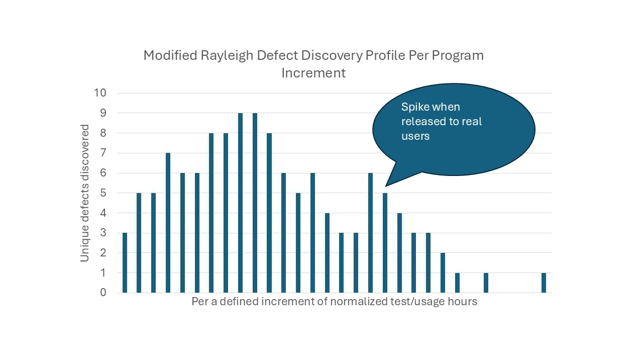
A modified Rayleigh defect discovery profile across a program increment — defects rise, peak, and decline through testing, then spike again once the software reaches real users.
What the class covers
Six modules, covered in a single self-guided day.
How to collect and analyze the software failure data
How to collect software failure data in a form that's actually usable for growth modeling, and how to do the initial analysis before fitting any model to it.
Every model in this class is only as good as the data behind it. Inconsistent collection produces a confident-looking forecast that's wrong.
How to estimate parameters for various models such as the exponential or logarithmic model
How to estimate the parameters of several reliability growth models — including exponential and logarithmic models — and compare which one actually fits your data.
No single model fits every data set. Knowing how to estimate and compare several is what keeps a forecast honest.
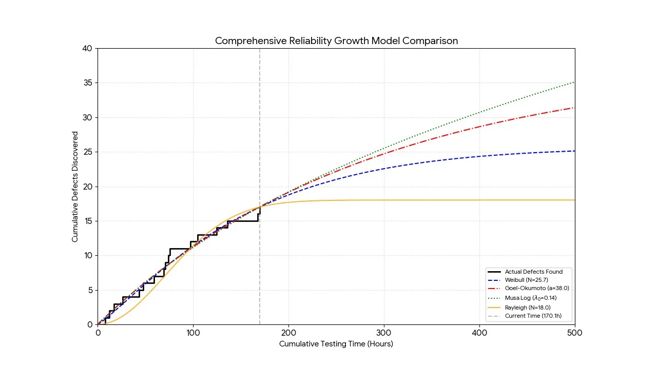
A comprehensive reliability growth model comparison: actual defects found against Weibull, Goel-Okumoto, Musa Logarithmic, and Rayleigh model fits — the same comparison this module teaches you to run.
How to estimate the software failure rate and MTBSF
How to turn a fitted growth model into a specific software failure rate and mean time between software failures (MTBSF) estimate.
A fitted curve is a means to an end. Failure rate and MTBSF are the numbers requirements and release decisions are actually written against.
How to forecast the estimates into the future
How to project the fitted model forward — beyond the current test data — to estimate reliability at a future point, such as planned release.
The number that matters isn't where reliability is today, it's where it's projected to be when the software actually ships.
How to determine how many defects need to be fixed, or how much more testing is needed
How to work backward from a reliability objective to a specific number of defects that still need fixing, or the additional test time needed to close the gap.
"Keep testing" isn't a plan. A specific number — defects or hours — is something a schedule can actually be built around.
How to make a release decision as per IEEE 1633 clause 5.5
A walkthrough of IEEE 1633 clause 5.5 — what it actually requires for a defensible release decision, and how the growth model outputs from this class feed directly into it.
Every module before this one exists to support this decision. This is where the forecast actually gets used.
Format, duration, and prerequisites
1 Day
Delivered as a single day of self-guided instruction.
Virtual, Self-Guided
Work through the material on your own schedule, at your own pace.
None Required
No prior class is required. Requs Trend is recommended but not required to own.
Turn raw failure data into a defensible release decision.
Register for the class, or schedule a demonstration of Requs Trend.